Fire Detection Based on Image Learning by Collaborating CNN-SVM with Enhanced Recall
This is an Open Access article distributed under the terms of the Creative Commons Attribution Non-Commercial License(https://creativecommons.org/licenses/by-nc/3.0/) which permits unrestricted non-commercial use, distribution, and reproduction in any medium, provided the original work is properly cited.
Abstract
Effective fire sensing is important to protect lives and property from the disaster. In this paper, we present an intelligent visual sensing method for detecting fires based on machine learning techniques. The proposed method involves a two-step process. In the first step, fire and non-fire images are used to train a convolutional neural network (CNN), and in the next step, feature vectors consisting of 256 values obtained from the CNN are used for the learning of a support vector machine (SVM). Linear and nonlinear SVMs with different parameters are intensively tested. We found that the proposed hybrid method using an SVM with a linear kernel effectively increased the recall rate of fire image detection without compromising detection accuracy when an imbalanced dataset was used for learning. This is a major contribution of this study because recall is important, particularly in the sensing of disaster situations such as fires. In our experiments, the proposed system exhibited an accuracy of 96.9% and a recall rate of 92.9% for test image data.
Keywords:
Vision sensing, Fire detection, Machine learning, Convolutional neural network (CNN), Support vector machine (SVM), Recall rate1. INTRODUCTION
Fire is one of the most common disasters that causes enormous losses of life and property. For example, in 2022, more than 40,000 fires occurred in the Republic of Korea, resulting in the deaths of 341 people [1]. To mitigate such incidents, sensing fires swiftly and accurately in their early states is of utmost importance.
Commercial fire sensors sold on the market include heat, smoke, and carbon monoxide (CO) detectors. These point detectors have several advantages, including low cost, simple technology, small size, and ease of installation. However, they are effective only for short indoor sensing distances. Moreover, the system manager must visit the fire alarm site in person to ascertain whether the alarm has been triggered by an actual fire or simply because of the malfunction of the sensor.
Vision is the most powerful sensory function in humans. As humans recognize the occurrence of fire using eyes, research and development have been undertaken to automatically detect fire occurrences using machine vision. If a vision system is used, the system manager can promptly assess the size and progress of a fire using real-time camera images when the fire breaks out. In addition, a practical advantage arises from the feasibility of installing and operating only fire-detection software on existing camera systems, obviating the need for additional sensing device installations.
With recent advances in machine vision technology, various attempts have been made to automatically detect fires using image processing [2,3]. Traditional vision-sensing and pattern-recognition technologies utilize the spatiotemporal characteristics of smoke or flames for detection. Pixel color is often used as an important fire detection cue. Recently, machine learning (ML), which utilizes deep neural networks (DNNs), has become one of the main approaches to automatic image classification. The widespread adoption of DNN-based ML is backed by high computing power using graphics processing units (GPUs) and large numbers of training images that are readily accessible through internet sources or datasets. Furthermore, many efficient ML methods and software tools have been competitively released during the ongoing surge in global AI research and development.
Among the various types of DNNs, the convolutional neural network (CNN) is widely used for image learning. A practical advantage of CNNs is their ability to automatically learn target features without requiring manual specifications. CNNs have demonstrated exceptional accuracy in diverse applications including fire sensing. For instance, Hao et al. [4] achieved a flame detection accuracy of 92.5% utilizing a CNN on the region of interest (ROI) extracted based on spatiotemporal image attributes. Zhong et al. [5] achieved an accuracy of 97.6% by training a CNN on ROIs derived using an RGB color model applied to video images. However, this approach has two limitations. First, the ROI selection may occasionally be incorrect. For instance, if a fire flame does not match a preselected color model, it remains undetected and is not processed by the CNN. Second, although numerous images can be acquired from several video clips of fires, the diversity of these images is often low. Therefore, there are doubts about whether a CNN trained with images from several video clips can work well in various real-world situations.
In this study, we use a CNN and support vector machine (SVM) that operate collaboratively for fire image detection. For the task of fire detection, we emphasize the importance of the recall rate, although many existing ML-based pattern-classification methods use accuracy as a major performance measure. In disaster situations, including fires, the detection of all target images is of great importance, and the recall rate represents this performance. The number of fire images used for learning can be significantly lower than the number of non-fire images, and this dataset imbalance results in a low recall of fire images when a CNN is used. We tackle this practical problem by employing an SVM, as the classification decision boundary of an SVM is determined not by the entire data but only by support vectors, the data that lie on the maximum margin hyperplanes in the feature space. In this case, the output of a CNN based on imbalanced data can be appropriately modified using an SVM. Linear and nonlinear SVMs with various parameters were tested and analyzed.
2. INTEGRATION OF CNN AND SVM FOR FIRE IMAGE DETECTION
An SVM classifier was employed to identify fire images based on feature vectors obtained by a CNN. SVMs have been used successfully in various fields. However, as reported in previous studies [6,7], the performance of an SVM generally does not reach that of a CNN. One reason for this is that it is difficult to appropriately select the image features required for training an SVM. Thus, we constructed a linked learning system that automatically extracts a large feature vector from an input image using a CNN and then classifies the image using an SVM based on the feature values.
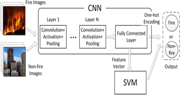
The structure of the proposed fire-image detection system is illustrated in Fig. 1. The learning operation of the system consisted of two steps. In the first step, a dataset of fire and non-fire images was used to train a CNN. In a CNN, the feature vector of the input image is obtained by performing a series of convolution and pooling operations. In the second step, an SVM was trained to classify the input images into fire or non-fire classes based on the feature values provided by the CNN. After the learning steps, a feature vector was obtained using the CNN for a given input image, and the SVM predicted the class of the input based on the features.
2.1 Image Feature Extraction using a CNN
A CNN is a deep neural network that is primarily used for image classification. The input of a CNN is a tensor consisting of the numbers, height, width, and channels of the image data. The convolutional operation between the input image and kernels is performed in the convolutional layer of the CNN, and then the output is computed using an activation function. The size of the output data can be reduced by using the maximum or average value of a window in the pooling layer to prevent overfitting. After extracting the features of an image through a series of convolutional and pooling layer operations, the feature values are flattened into a vector. The feature vector is then propagated through multiple fully connected layers, and the result is obtained using the softmax operation. Finally, one-hot encoding is performed. If the output of such a feedforward operation differs from the actual label of the image, the supervised learning process for modifying the parameters of the neural network through backpropagation is repeated until the desired output is obtained.
In this study, the input of the CNN was RGB color images, which were 224 × 224 pixels in size. After repeating the convolution and max-pooling operations four times with 3 × 3 kernels and a 2 × 2 pooling window, a feature vector with 4,608 elements was generated. In the fully connected network, the size of the feature vector was reduced to 256, and the vectors were connected to the output nodes. The activation function used in each layer was ReLU.
2.2 Classification by an SVM
An SVM is a supervised machine learning model that is useful for data classification. A two-class data classification problem using an SVM is described in Eq. (1) [8,9].
| (1) |
where x is the N-dimensional training data, ϕ(x) is a feature-space transformation, and b is a bias term. When the target output for a given input is ti ∈ {-1, +1}, i=1, …, N, w and b are determined such that the output becomes y(xi)>0 for ti=+1 and conversely y(xi)>0 for ti=-1. An SVM selects the decision boundary to maximize the margin between two classes. This decision boundary in the feature space is determined not by all the training data, but only by the support vectors.
| (2) |
| (3) |
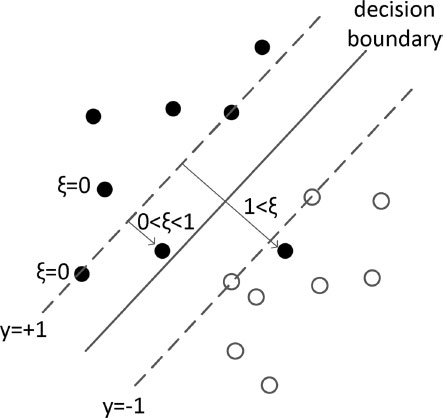
The aforementioned SVM model is suitable for datasets that can be completely separated. However, in practice, data often have a complex distribution, and it is difficult to separate them perfectly using a straight line in the feature space. Therefore, by acknowledging the existence of data misclassified by a decision boundary, a slack variable ξi=|ti-y(xi)| is introduced to impose a penalty on misclassified data. The target function to be minimized is set as follows:
| (4) |
where C>0 is a parameter that controls the tradeoff between the slack variable penalty and the decision margin. Fig. 2 shows the SVM classifier and the slack variable.
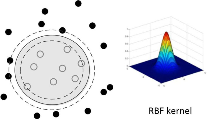
If a given classification problem is nonlinear, as shown in Fig. 3, an SVM model using a linear kernel does not perform well. In this situation, it can be effective to use a radial basis function (RBF) presented in Eq. (5) as the kernel for nonlinear learning.
| (5) |
where γ is the kernel parameter. Setting a small value of γ reduces the curvature of the decision boundary, thereby preventing overfitting. In a complex nonlinear data distribution, on the other hand, γ must be increased. When using an SVM with a linear kernel, the best result is found by varying parameter C n times. In comparison, when using an SVM with an RBF kernel, for finding the best γ, search must be conducted an extra m times, i.e., n×m grid search is needed.
2.3 Dataset Imbalance and Performance Measure
The ML performance depends heavily on the quality of the dataset used. Erroneous, irrelevant, or insufficient data affect the accuracy of learning, and there is a high possibility of incorrect predictions in utilization after learning. However, it is difficult to construct a suitable dataset for many real-life situations. A practical problem is that the amount of data for a particular class is often significantly smaller than that for another class. This is known as the data imbalance problem [10].
In the case of ML for vision-based fire sensing, acquiring images of various fire states under all possible conditions is virtually impossible. The background scene varies from place to place, and fire images may vary even in the same place depending on the season, weather, time, and cause of the fire. Even if all these conditions are assumed to be fixed, the image varies rapidly depending on the progress of the fire. In contrast, non-fire images can be easily collected as required. When the number of non-fire images is much larger than the number of fire images in a training dataset, the ML system learns more from the non-fire images than from the fire images.
In ML-based classification, the accuracy defined in Eq. (6), is typically used as the learning performance indicator.
| (6) |
where TP means true positive, TN means true negative, FP means false positive, FN means false negative, and symbol # means “number of.” Although accuracy is important in ML, measuring the performance of a model using accuracy is problematic in some cases. For example, it was pointed out that accuracy-based machine learning can lead to practical problems in fire detection because the reliability of the automated fire alarm system will be lowered if the false alarm rate is high [11].
We believe that, in the case of disaster sensing, including fires, the ability of a model to detect a target without failure is of great importance. This ability can be measured using the recall rate, defined in Eq. (7). The recall of a system should be checked, particularly if there is an imbalance in the dataset. As a simple example, for an imbalanced training dataset consisting of 100 fire images and 900 non-fire images, if the detection system simply determines that all images belong to the majority (non-fire), the accuracy of the system is 900/1000 = 0.9. However, the recall of fire image detection is 0/100 = 0.
| (7) |
3. RESULTS OF THE PROPOSED HYBRID METHOD USING CNN AND SVM
3.1 Image Dataset and Classification Results of CNN
A CNN was constructed as described in Section 2.1. To train the CNN, we used an image dataset from Kaggle [12] that contained 756 fire images and 243 non-fire images. However, the actual number of fire images used in our experiments was 751, after excluding five large watermarked or significantly edited images. To diversify and enrich the non-fire image data, natural and artificial landscape images from MIT CSAIL [13] were added. The MIT CSAIL dataset consists of images from eight categories: tall buildings, inside cities, streets, highways, coasts, open countries, mountains, and forests. The total number of non-fire images we used in our experiment was 2,931.
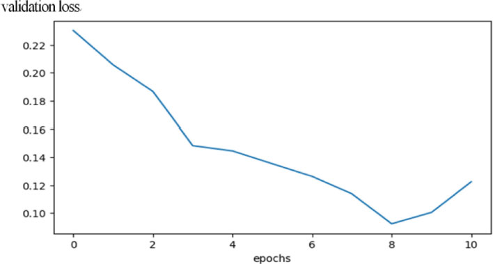
The dataset images in the RGB color format were used as inputs to the CNN after converting them into 224×224-pixel images. The image dataset was divided in the ratio of 60%:20%:20% for training, validation, and testing. The experiment was repeated five times using randomly shuffled data. The adaptive moment estimation (ADAM) method was used for optimization. The batch size was set to 32, and learning was stopped when the loss for the validation data increased. Fig. 4 shows an example of the training of the CNN, where the minimum loss occurs at the 8th epoch; thus, the model parameters at this time are saved and used in the test.
The CNN constructed in this study exhibited a fairly high classification accuracy of 96.0[%] on average for the test images, as shown in Table 1. However, if the individual recall rates for fire and non-fire images are compared, the recall for fire images is only 88.8% on average, which is much lower than the 97.8% recall for non-fire images. This indicates that the training of the CNN occurred mostly on non-fire images because of the imbalance in the dataset. In particular, in the experiment with Data Combination 4, the recall rate for the fire images was quite low; however, the average accuracy was still high because of the numerous correctly classified non-fire images. This is not the objective of fire detection. If we consider only the learning accuracy as a performance index, as in many existing studies, it is easy to overlook this situation, which can lead to dangerous results in the automatic sensing of disasters, such as fires, when the system is employed in real-life applications.

Performance of CNN (The dataset was shuffled randomly five times and divided into 60%, 20%, and 20% for training, validation, testing)
For comparison purposes, the dataset was divided into 70%, 15%, and 15% for training, validation, and testing, respectively, and the experimental results are listed in Table 2. These results are similar to the results presented in Table 1.
3.2 Results of SVM Classification
Linear and nonlinear SVMs were tested to classify the input images based on the feature vectors extracted by the CNN. First, an SVM with a linear kernel was considered. A total of 256 feature values were used. With the dataset used in the experiment shown in Table 1, the SVM performance was determined for different values of parameter C in Eq. (4). For example, with Data Combination 1, the performance of the SVM according to the variation of C was as shown in Table 3, where C = 1×10³ yields the best value. When the SVM was used for other data combinations in the same manner, the results shown in Table 4 were obtained. Compared to the results of the CNN shown in Table 1, the test accuracy increased slightly from 96.0% to 96.9%, and the recall increased significantly from 88.8% to 92.9% on average. This demonstrates that the proposed linked structure of the CNN and SVM is useful for improving the recall rate for a dataset with a relatively small number of fire images while maintaining accuracy.
Subsequently, the performance of a nonlinear SVM using an RBF kernel was evaluated. A grid search for optimal parameters was performed, and the search results for Data Combination 1 are listed in Table 5, where C = 1×10³ and γ = 10 are the best parameter values. In this manner, the optimal parameter values were determined for other data combinations, and Table 6 shows the experimental results of using an RBF SVM. When comparing Table 6 with Table 1, which was obtained using the CNN, the combination of the RBF SVM with the CNN showed a slightly higher accuracy and significantly improved recall. However, its performance was similar to that of a linear SVM (Table 4), although the training procedure for the nonlinear SVM was more complex.

Accuracy of CNN + RBF SVM for different parameter values for the validation data of Data Combination 1
4. CONCLUSIONS
In this paper, we present a hybrid machine-learning technique for image-based fire sensing. The proposed approach involves a structured process in which extensive features are extracted from input images using a CNN, followed by SVM-based classification.
This study contributes to ML-based visual fire sensing in two ways. First, the proposed method significantly enhances the recall performance of fire-image learning. When the number of fire images in a dataset is relatively limited, the conventional practice of using accuracy as the primary performance metric becomes problematic in real-world applications, particularly in the automated detection of disasters such as fires. Through experiments, we demonstrated the efficacy of incorporating an SVM to address the challenge of imbalanced training data, leading to a substantial improvement in the recall rate for fire image detection. Notably, our proposed method holds practical significance because it enables increased recall without compromising accuracy.
The second main contribution of this study is the exploration of SVMs with both linear and nonlinear kernels. A comparative analysis showed that the linear SVM demonstrated good performance. In our empirical evaluations using a dataset with 3,682 images, including 751 fire images, the integration of a linear SVM with a CNN resulted in an accuracy of 96.9% and a recall of 92.9%, whereas the CNN alone achieved 96.0% accuracy and 88.8% recall. Similar results were obtained when an RBF-SVM was tested. However, the process of searching for the optimal parameter values of an RBF SVM is more complex than that of a linear SVM.
In conclusion, the combination of a CNN and a linear SVM is effective for fire image detection. The proposed approach addresses recall-related challenges associated with imbalanced data. The empirical results underscore the practical utility of this method in automated fire detection, where increased recall without undermining accuracy is highly important.
Acknowledgments
This research was supported by the Daegu University Research Grant, 2019.
REFERENCES
- https://nfds.go.kr/dashboard/status.do, (retrieved on Jun. 28, 2023).
-
S. Geetha, C. S. Abhishek, and C. S. Akshayanat, “Machine vision based fire detection techniques: A survey”, Fire Technol., Vol. 57, No. 2, pp. 591-623, 2021.
[https://doi.org/10.1007/s10694-020-01064-z]

-
F. Bu and M. S. Gharajeh, “Intelligent and vision-based fire detection systems: A survey”, Image Vis. Comput., Vol. 91, p. 103803, 2019.
[https://doi.org/10.1016/j.imavis.2019.08.007]

-
X. Hao, C. Linhu, and H. Weixin, “Video flame detection using convolutional neural networks”, Proc. IEEE 4th Int. Conf. on Image, Vision and Comput. (ICIVC), pp. 539-543, Xiamen, China, 2019.
[https://doi.org/10.1109/ICIVC47709.2019.8981110]

-
Z. Zhong, M. Wang, Y. Shi, and W. Gao, “A convolutional neural network-based flame detection method in video sequence”, Signal Image Video Process., Vol. 12, pp. 1619-1627, 2018.
[https://doi.org/10.1007/s11760-018-1319-4]

-
M. Balipa, P. Shetty, A. Kumar, B. R. Puneeth, and Adithya, “Arecanut disease detection using CNN and SVM algorithms”, Proc. Int. Conf. on Artif. Intell. and Data Eng. (AIDE), pp. 01-04, Karkala, India, 2022.
[https://doi.org/10.1109/AIDE57180.2022.10060130]

-
K. Myagila and H. Kilavo “A comparative study on performance of SVM and CNN in Tanzania sign language translation using image recognition”, Appl. Artif. Intell., Vol. 36, No. 1, pp. e2005297(1)-e2005297(16), 2022.
[https://doi.org/10.1080/08839514.2021.2005297]

- C. M. Bishop, Pattern Recognition, and Machine Learning, Springer, New York, 2006.
- A. Hertzmann, D. J. Fleet, and M. Brubaker, Machine Learning and Data Mining Lecture Notes, Dept. of Computer and Mathematical Sciences, Univ. of Toronto, Scarborough, 2015.
-
P. Kumar, R. Bhatnagar, K. Gaur and A. Bhatnagar, “Classification of imbalanced data: Review of methods and applications”, IOP Conf. Ser. Mater. Sci. Eng., Vol. 1099, No. 1, pp. 012077(1)-012077(9), 2021.
[https://doi.org/10.1088/1757-899X/1099/1/012077]

-
A. M. Fernandes, A. B. Utkin, and P. Chaves, “Automatic early detection of wildfire smoke with visible-light cameras and EfficientDet”, J. Fire Sci., Vol. 41, No. 4, pp. 122-135, 2023.
[https://doi.org/10.1177/07349041231163451]

- https://www.kaggle.com/datasets/phylake1337/fire-dataset, (retrieved on Feb. 12, 2023).
- https://people.csail.mit.edu/torralba/code/spatialenvelope, (retrieved on Mar. 15, 2023).


