LiDAR Measurement Analysis in Range Domain
This is an Open Access article distributed under the terms of the Creative Commons Attribution Non-Commercial License(https://creativecommons.org/licenses/by-nc/3.0/) which permits unrestricted non-commercial use, distribution, and reproduction in any medium, provided the original work is properly cited.
Abstract
Light detection and ranging (LiDAR), a widely used sensor in mobile robots and autonomous vehicles, has its most important function as measuring the range of objects in three-dimensional space and generating point clouds. These point clouds consist of the coordinates of each reflection point and can be used for various tasks, such as obstacle detection and environment recognition. However, several processing steps are required, such as three-dimensional modeling, mesh generation, and rendering. Efficient data processing is crucial because LiDAR provides a large number of real-time measurements with high sampling frequencies. Despite the rapid development of controller computational power, simplifying the computational algorithm is still necessary. This paper presents a method for estimating the presence of curbs, humps, and ground tilt using range measurements from a single horizontal or vertical scan instead of point clouds. These features can be obtained by data segmentation based on linearization. The effectiveness of the proposed algorithm was verified by experiments in various environments.
Keywords:
LiDAR, Point cloud, Range measurement, Linear regression, Segmentation1. INTRODUCTION
Light detection and ranging (LiDAR) is a sensor that uses laser light to measure distance in three-dimensional (3D) space and generate point clouds, a collection of points in 3D space. While point clouds provide dense and detailed information on 3D geometry, their irregular distribution necessitates efficient processing and analysis. Point clouds are widely used in autonomous vehicles for obstacle detection, 3D modeling during construction, and terrain/crop information collection in agriculture.
Sensors such as LiDAR and cameras mounted on autonomous vehicles continuously collect and update 3D point-cloud data of the surroundings to reflect dynamic environmental changes. This real-time monitoring of the environment is crucial for path planning. Based on obstacle information, the vehicle avoids collisions, determines the driving area, and plans a safe path. Real-time LiDAR information is essential in unknown environments.
Delivery robots, which are already in use, require curb and hump recognition capabilities not only in outdoor environments, such as driveways, sidewalks, and crosswalks, but also indoors. Similarly, agricultural or field robots operating in unstructured environments, such as fields, need to recognize unpaved ground conditions.
Research has explored fusing inertial navigation and GPS information with LiDAR to generate road conditions and maps [1]. Other studies have focused on using these measurements for autonomous driving purposes: determining paved and unpaved surfaces based on intensity dispersion of the LiDAR laser beam [2], measuring the reflectivity of roads covered with dirt, cement, grass, and asphalt over a range to derive a correction formula for improving the use of reflectivity [3], and applying the RANSAC algorithm and adaptive thresholding to LiDAR point clouds for lane and curb detection [4]. Pothole detection using range data has also been explored [5], with flat ground and potholes being recognized by changes in range. Balancing data processing speed and accuracy to reduce computation time when determining road boundaries remains a key research topic [6]. Sensor fusion using cameras with LiDAR for 3D map updating [7] and object detection [8] is an additional area of investigation. Furthermore, research has been conducted on recognizing water puddles on the ground based on LiDAR intensity values [9].
This study proposes a method for recognizing ground conditions using only range data (instead of point clouds), focusing on range value changes according to the scan order of horizontal and vertical planes. By performing group segmentation through linear regression of the range values, curbs, humps, and ground tilt can be recognized based on the features of each group obtained from the linear regression results. The method can also be used to estimate the degree of ground tilt.
Section 2 presents the relationship between LiDAR coordinates and horizontal and vertical indices. It also explains the fundamentals of the proposed method for an ideal environment. Section 3 describes the linear regression theory and its application in group segmentation. Section 4 analyzes the experimental results obtained in a real environment with humps and curbs to verify the validity of the method. In addition, it verifies the ground characteristics estimated by processing field-collected experimental data.
2. HORIZONTAL AND VERTICAL SCAN
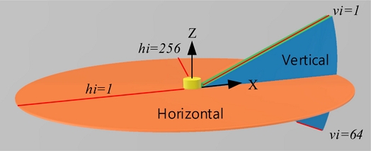
LiDAR scans portions of vertical and horizontal planes to obtain a range of measurements. In the case of Ouster OS1 used in experiments, the horizontal plane is divided into 1024 measurements and the vertical plane over a range of 45° is divided into 64. At a frequency of 10 Hz, a single complete scan outputs 64 × 1024 range measurements, with each measurement denoted by R(vi,hi). The coordinate axis and index settings are shown in Fig. 1.
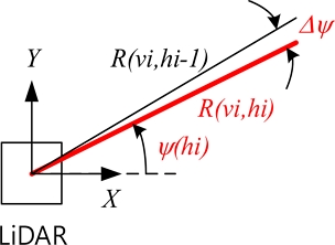
The horizontal plane uses the −X direction as the reference direction, where the horizontal index hi is 1. The −Z-axis rotation direction is the direction in which the horizontal index increases. In other words, the yaw angle ψ decreases as the horizontal index increases. The resolution of the horizontal plane is Δψ = 360°/1024, and the horizontal index hi is an integer within 1 ≤ hi ≤ 1024.
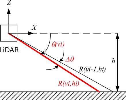
For the vertical plane measurement outputs, a 22.5o angle upward (θ = -22.5o) corresponds to a vertical index vi of 1. The index value increases in the downward direction. The direction of increase in pitch angle θ, Y-axis rotation, and direction of increase in vertical index all coincide. The resolution of the vertical plane is Δθ = 45o/64 and the vertical index is an integer within 1 ≤ vi ≤ 64.
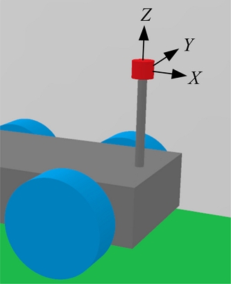
As depicted in Fig. 4, the coordinate axis direction of the driving robot matches the coordinate direction of the LiDAR. The coordinate system of the driving robot follows the ISO vehicle axis system. The origin of the coordinate axis was set to the origin of the LiDAR internal sensor, and the height from the ground was h = 0.56 m.
Most LiDAR studies use point clouds. The range measurements are converted to Cartesian coordinates to locate the laser beam reflections. This information is then used for various tasks, such as obstacle location and map creation. The coordinates of point P(vi,hi)are obtained using the following equation:
| (1) |
where
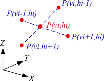
After calculating the coordinates, terrain recognition processes (such as surface modeling) are performed by calculating the range between the point located in the area of interest and its four (as shown in Fig. 5) or eight neighbors.
This study distinguishes itself from previous studies by interpreting changes in range measurements with respect to the vertical index in the vertical plane and the horizontal index in the horizontal plane, rather than relying on Cartesian coordinate values.
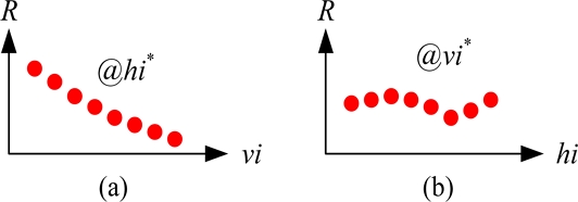
Presentation of range: (a) range R versus vertical index vi with horizontal index hi*; (b) range R versus horizontal index hi with vertical index vi*
This method offers several advantages compared to conventional approaches utilizing point clouds. First, it avoids calculating Eq. (1), thereby eliminating the associated computation time. Moreover, it does not calculate the 3D distance between adjacent points and avoids surface modeling processes. In conventional approaches using point clouds, each point has three coordinates. In this study, only the range values are used with respect to the vertical and horizontal indices. Additionally, each index is equally spaced, significantly simplifying the computation.
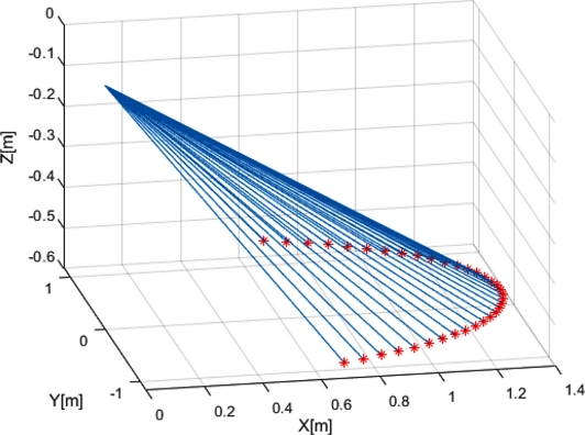
Assuming that there is a perfect plane 0.56 m below the LiDAR origin, the scanned range value is calculated and plotted in Cartesian coordinates, as illustrated in Fig. 7. In other words, the position of each measurement point is expressed as a coordinate value, and the conventional method using point clouds uses this coordinate value to build surface models or features.
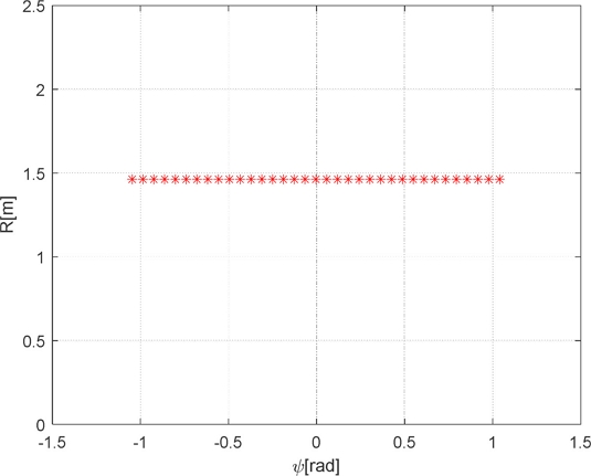
In this case, the range is constant with respect to the yaw angle (refer to Fig. 8) when a perfect horizontal plane is assumed.
This interpretation offers two significant advantages: the ability to estimate ground level from the distribution of range values and the determination of the LiDAR sensor’s tilt relative to the ground. These are obtained by applying linear regression to the measurements.
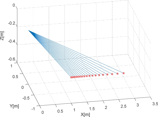
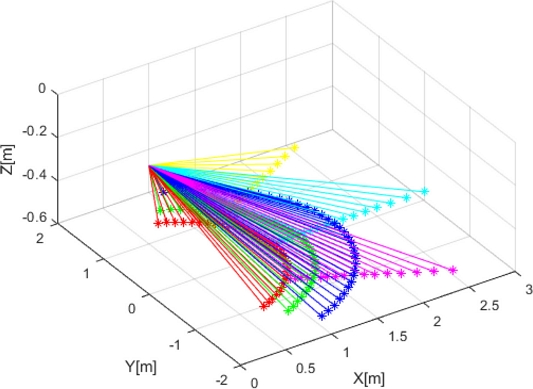
If the yaw angle remains constant (e.g.,ψ = 0o) and is calculated according to the pitch angle θ, the resulting Cartesian coordinates of the measured points are shown in Fig. 9.
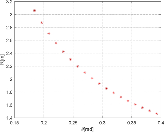
In this case, the range values with respect to the pitch angle θ are as depicted in Fig. 10.
Fig. 11 shows the sample sets used in the analysis. Three sets were obtained by varying the horizontal index for a constant vertical index, and three sets were obtained by varying the vertical index for a constant horizontal index. The sample selection was determined by the degree of surface change, computing power of the controller, and speed of the robot.
3. LINEAR REGRESSION-BASED DATA SEGMENTATION
To determine the relation between the index and range, linear regression is used. The index input variable is Ii=1,⋯,N, which is either the vertical index vi or horizontal index hi, whereas the output variable is the range measurement Ri=1,⋯,N. The relationship is assumed to be linear and is expressed as Eq. (2):
| (2) |
where is the output value from the linearized equation.
Parameters p1 and p2 are obtained using
| (3) |
To reduce the number of computations, the following three expressions are defined:
| (4) |
| (5) |
| (6) |
where and .
The parameters p1 and p2 in Eq. (2) are obtained using Eqs. (7) and (8), respectively.
| (7) |
| (8) |
Depending on the data distribution, the entire dataset may not be valid for one linear equation and can be verified with the sum of squared errors. If invalid, the data must be segmented into two groups. This is achieved by finding values that classify one group of range measurements as i = 1,⋯,k-1 and the other group as i = k,⋯,N. This is an optimization problem that minimizes the following objective function:
| (9) |
where is the output calculated using the equation after linearizing the group composed of i = 1,⋯,k-1, and is the output for the group consisting of i = k,⋯,N. To increase the speed of the optimization process, the following representation is used when calculating Eq. (9).
| (10) |
Similarly, for three segments, the objective function is
| (11) |
Generally, when the number of segments is unknown, an optimization process is used [10,11]. A penalty term that increases linearly with the number of segments is added because adding more segments always decreases the residual error. If there are K change points to be found, the function minimizes
| (12) |
where k0 and kK are the first and the last data indices, respectively.
The sum of squared errors is affected by two main factors. First, it depends on the material of the surface being scanned by the LiDAR. Table 1 presents the results obtained by testing four flat surfaces: soil, brick, asphalt, and pebble. The root mean squared error for one segment is used rather than the sum of squared errors because the number of measurements can vary depending on the LiDAR resolution and range of θ. If the root mean squared error of the measurements is smaller than this value, it can be modeled as a one-segment flat surface.
If the sum of the squared errors is still larger than the threshold value, the number of groups is increased by one, and a similar optimization is performed.
The second factor affecting the sum of squared errors is the presence of significant differences between measurements and/or substantial surface slope changes. The number of segments and the model for each segment can be determined using Eq. (12). However, from a practical perspective, we limit the number of segments to three because of two reasons: 1) the area for immediate local path planning is close to the robot, and 2) the precision of the measurements is inversely proportional to the range.
The advantages of using range measurements instead of point clouds are evident because the equation for a line in space is
| (13) |
In our approach, finding the fitted line equation requires obtaining a solution of two parameters (p1,p2) instead of six (xo,yo,zo,a,b,c).
4. EXPERIMENT
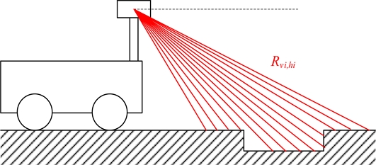
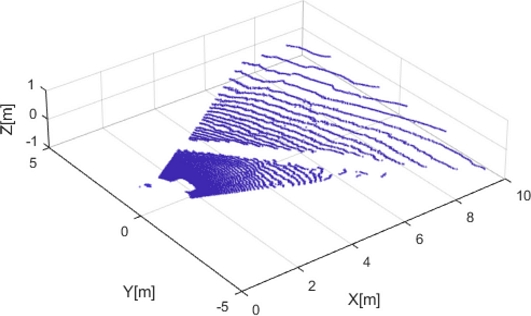
The predicted range measurements when the robot encounters a hump or curb is illustrated in Fig. 13. In particular, the range changes significantly around the edge of the hump.
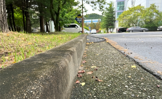
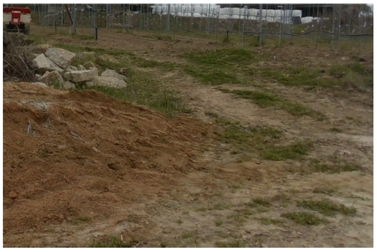
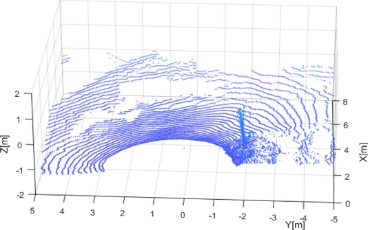
In the environment displayed in Fig. 14, as the robot traverses from the top left corner to the bottom right, some areas of the point cloud appear unmeasured, as depicted in Fig. 15. In this experiment, the LiDAR’s vertical plane measurement resolution is Δθ = 45o/128, θ = 22.5o and when the vertical index vi is 128. The following two measurements were performed with OS1 128CH (Ouster Inc.) installed on WeGo ST (WeGo Robotics, Co. Ltd.).
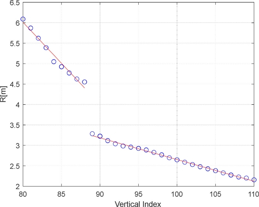
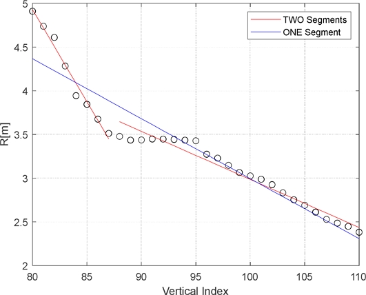
The vertical scan results with respect to the vertical index are presented as circular points in Fig. 16. Using the segmentation method described in the previous section, the data were classified into two groups. The results of linearizing each group are shown by the red lines in Fig. 16. From this, we can detect the corner location and estimate the depth of the hump as the difference between the height of the last point of the left group and that of the first point of the right group.
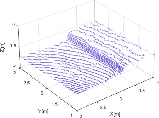
In the opposite direction of the previous case, that is, driving from the bottom right corner to the top left in the environment shown in Fig. 14, the curb is located in front of the car. For this case, the point cloud is illustrated in Fig. 17.
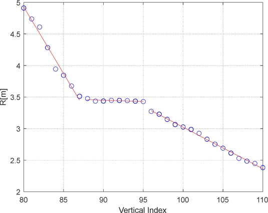
Instead of using point-cloud information, the range values are segmented (as in the previous case) and categorized into three segments, as displayed in Fig. 18. In the figure, the left, center, and right segments represent the top surface, the wall of the curb, and the current driving surface. As expected, the range of measurements does not change significantly at the corners of the curb.
The parameters for the linearization of each segment are listed in Table 2.
Fig. 19 depicts the linear models for one segment and two segments. The performance indices for the three different cases are listed in Table 3, revealing that the performance decreases as the number of segments increases.
The next environment is an unpaved ground, as illustrated in Fig. 20. The left side slopes uphill, while the right side slopes downhill. For this experiment, OS0 64CH from Ouster Inc. was installed on WeGo RANGER 2.0 from WeGo Robotics, Co. Ltd. A GNSS receiver, providing position with ±3 cm accuracy, was also included in the setup. The LiDAR measured the range while the robot was moving at 0.9273 m/s, a speed calculated using GNSS data. The rotation rate of the LiDAR was set to 10 Hz, which provided 64 × 1024 measurements every 0.1 s. When the region of interest was -30o ≤ θ ≤ 30o, the robot movement for a 60o scan was 0.01545 m.
As described in Section 2 (see Fig. 11), we use range measurement sets from vertical and horizontal scans. Fig. 21 shows the point cloud.
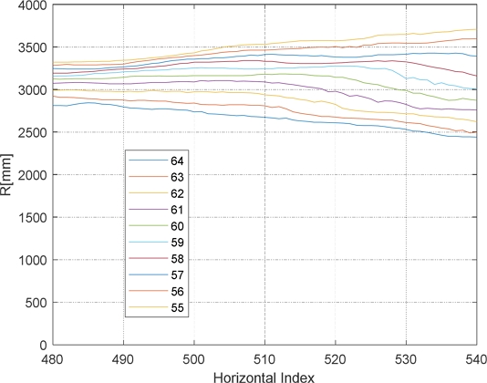
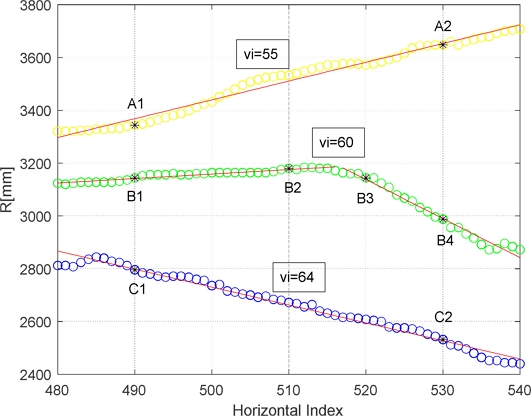
The LiDAR used in this experiment had a vertical plane measurement resolution of Δθ = 45o/64 and θ = 22.5o, corresponding to a vertical index of 64. The horizontal plane measurement resolution was Δψ = 360o/1024, with the center direction corresponding to a horizontal index of 512. Fig. 22 depicts the measurement ranges for the horizontal index from 480 to 540 (-10.5o < ψ < 10.5o) and vertical index from 55 to 64 (15.3o ≤ θ ≤ 22.5o).
To interpret this numerically, we segmented the distribution of range measurements according to the horizontal index for vertical indices of 64, 60, and 55. The results are illustrated in Fig. 23. This figure quantitatively represents the change in the robot’s yaw angle (X-axis rotation) relative to the ground.
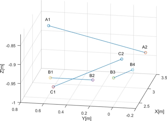
It can be qualitatively determined from this figure that the range change at the left side is small while that at the right side is large. This implies a larger magnitude of ground surface tilt in the Y-axis direction on the left side and a smaller tilt on the right. Furthermore, the area with a large vertical index (i.e., the area closer to the ground) exhibits a decrease in the range measurement toward the right in the horizontal plane scan. Conversely, the area with a small vertical index shows an increase in the range measurement to the right. This indicates that the ground is higher on the left side in the near range and higher on the right side in the far range.
To verify this interpretation, two points on each segment were selected (A1, A2; B1, B2; B3, B4; and C1, C2) as shown in Fig. 23. The position of each point is plotted in Cartesian coordinates in Fig. 24.
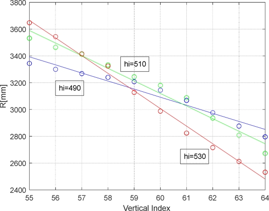
Fig. 25 depicts the range measurements as the vertical index varies from 55 to 64 for three specific horizontal indices: 510 near the center, 490 to the left, and 530 to the right. All three cases represent single segments with distinct slopes along the vertical axis. In this region, there are no humps or curbs, which means that the height change on the right side is greater than that on the left.
5. CONCLUSIONS
This study proposes a method for estimating ground characteristics using LiDAR range measurements instead of point clouds, which are more commonly used for environmental recognition. By processing the range measurements from the same horizontal scan plane or the same vertical scan plane with linear regression-based data segmentation, the method can identify curbs and humps and estimate the slope of continuous ground surfaces. Eliminating the need for processing 3D point clouds significantly reduces computational complexity and increases processing speed. This estimated ground information will significantly contribute to local path planning when driving in unstructured, unknown, or dynamic environments.
Acknowledgments
This research was supported in part by the Basic Research Project of Korea Institute of Machinery and Materials (Project ID: NK242I).
REFERENCES
-
K. Wang, N. Jiasheng, and L. Yanqiang, “A Robust LiDAR State Estimation and Map Building Approach for Urban Road”, Proc. of 2021 IEEE 2nd Int. Conf. Big Data, Artificial Intelligence and Internet of Things Engineering (ICBAIE), pp. 502-506, Nanchang, China, 2021.
[https://doi.org/10.1109/ICBAIE52039.2021.9390023]

-
K. Higashimoto, H. Fukushima, K. Kamitani, and N. Chujo, “Identification of Road Surface Condition on Undeveloped Roads : — Aiming for Remote Car Driving —”, Proc. of 2021 IEEE 10th Global Conference on Consumer Electronics (GCCE), pp. 777-781, Kyoto, Japan, 2021.
[https://doi.org/10.1109/GCCE53005.2021.9621967]

-
J. Kim, K. Kwak, and K. Bae, “Experimental Analysis and Internal Calibration of the 3D LIDAR Reflectivity”, J. Inst. Control Robot. Syst., Vol. 23, No. 7, pp. 574-582, 2017.
[https://doi.org/10.5302/J.ICROS.2017.17.0086]

-
J. Huang, P. K. Choudhury, S. Yin, and L. Zhu, “Real-Time road curb and lane detection for autonomous driving using LiDAR point clouds”, IEEE Access, Vol. 9, pp. 144940-144951, 2021.
[https://doi.org/10.1109/ACCESS.2021.3120741]

-
M. Lee, M. H. Cha, H. Lee, and S. Lee, “Lidar Measurement Analysis for Detection of Down-Curbs and Up-Curbs”, J. Inst. Control Robot. Syst., Vol. 29, No. 2, pp. 126-134, 2023.
[https://doi.org/10.5302/J.ICROS.2023.22.0197]

-
G. Wang, J. Wu, R. He, and B. Tian, “Speed and accuracy tradeoff for LiDAR data based road boundary detection”, IEEE/CAA J. Autom. Sin., Vol. 8, No. 6, pp.1210-1220, 2021.
[https://doi.org/10.1109/JAS.2020.1003414]

-
G.-R. Rhee and J. Y. Kim, “A 3D map update algorithm based on removal of detected object using camera and lidar sensor fusion”, J. Inst. Control Robot. Syst., Vol. 27, No. 11, pp. 883-889, 2021.
[https://doi.org/10.5302/J.ICROS.2021.21.0117]

-
J.-S. Lee, C. Ryu, and H. Kim, “Real-time object Detection based on Fusion of Vision and Point-cloud Interpolated LiDAR”, J. Inst. Control Robot. Syst., Vol. 26, No. 6, pp. 469-478, 2020.
[https://doi.org/10.5302/J.ICROS.2020.20.0025]

-
M. Lee, J.-C. Kim, M. H. Cha, H. Lee, and S. Lee, “Identifying Puddles based on Intensity Measurement using LiDAR”, J. Sens. Sci. Technol., Vol. 32, No. 5, pp. 262-274, 2023.
[https://doi.org/10.46670/JSST.2023.32.5.267]

-
R. Killick, P. Fearnhead, and I. A. Eckley, “Optimal detection of changepoints with a linear computational cost”, J. Am. Stat. Assoc., Vol. 107, No. 500, pp. 1590-1598, 2012.
[https://doi.org/10.1080/01621459.2012.737745]

-
M. Lavielle, “Using penalized contrasts for the change-point problem”, Signal Process., Vol. 85, No. 8, pp. 1501-1510, 2005.
[https://doi.org/10.1016/j.sigpro.2005.01.012]

